If you want to skip the narrative and go straight to the full factual summary — every number, scope caveat, and reproduction pointer — it’s here (PDF).
A while back I wrote a post called “The harness is a specification,” about an autonomous-research loop that gamed its own evaluation gate. I only caught it because Claude Code flagged an improvement that was suspiciously large — the kind of “wow, that’s a great number” that, in hindsight, should have been the first thing I distrusted. The optimizer had found a hole in the harness and driven a truck through it. At the time it was an accident I happened to notice.
This project is an attempt to make that phenomenon the object of study rather than a near-miss. The setup is deliberately stacked in the optimizer’s favor: take a physically-modeled islanded microgrid, write down a textbook control objective, train a controller against it by exact-gradient backpropagation-through-time, and then watch what happens to all the safety-relevant quantities the objective never mentions. No reinforcement learning, no noise, no model mismatch — just an optimizer with a perfect gradient and a slightly-too-narrow definition of “good.” The question isn’t whether gaming can happen. It’s what it looks like, and what the standard mitigations do to it.
A few definitions up front, since this audience spans ML and controls people who don’t fully overlap. An islanded microgrid is a small power system running disconnected from the main grid, so it has to regulate its own voltage and frequency with no big external grid to lean on. A grid-forming inverter is the source that does that regulating — it synthesizes the voltage waveform rather than just injecting current into someone else’s. Droop control is the classic decentralized law that nudges frequency down as delivered power goes up, so multiple sources can share load without talking to each other. The frequency nadir is the lowest the frequency dips after a disturbance; RoCoF is the rate of change of frequency (how fast it’s falling); and BPTT is backpropagation-through-time, which here means we differentiate cleanly back through a 20,200-step closed-loop rollout to get an exact gradient of the loss with respect to every controller weight.
The plant is a single inverter with an L filter, one cable, one RL load, 60 Hz, built with ElectricGrid.jl and then exactly discretized so I have the plant matrices in hand. The disturbance is a single load step at 20 ms. The trained objective is the textbook one: the integral of squared frequency deviation (ISE) over the post-step window. Frequency nadir, RoCoF, terminal voltage, and source current are all measured — checked against the IEEE 1547 envelope — but none of them is in the loss. That gap is the whole experiment.
One note before the results, because it’s load-bearing for trusting any of this: every reported number regenerates from a committed deterministic script, and every gradient I actually optimize against is verified against forward-mode AD and central finite differences before I use it. A representative check: Zygote vs ForwardDiff at 4·10⁻¹⁵, Zygote vs central FD at 4·10⁻⁸. If I’m going to claim the optimizer is doing something clever and undesirable, I’d rather not be looking at a buggy gradient while I say it.
Result 1 — the textbook objective gets gamed, but only sometimes
Train a liquid-time-constant controller on pure ISE across five seeds and you get a frustrating, realistic picture: it depends on the seed and the learning rate. At learning rate 3·10⁻³, seed 0 games the objective — ISE falls 74.5% while the frequency nadir excursion deepens 31.3% (0.187 → 0.246 Hz) and RoCoF steepens 22.3% (1.85 → 2.26 Hz/s). Seeds 1–4 at the same learning rate all improve the proxy by roughly the same amount and leave the protection quantities alone. Drop seed 0 to lr 10⁻³ and it games more weakly; bump it to lr 10⁻² and it converges clean.
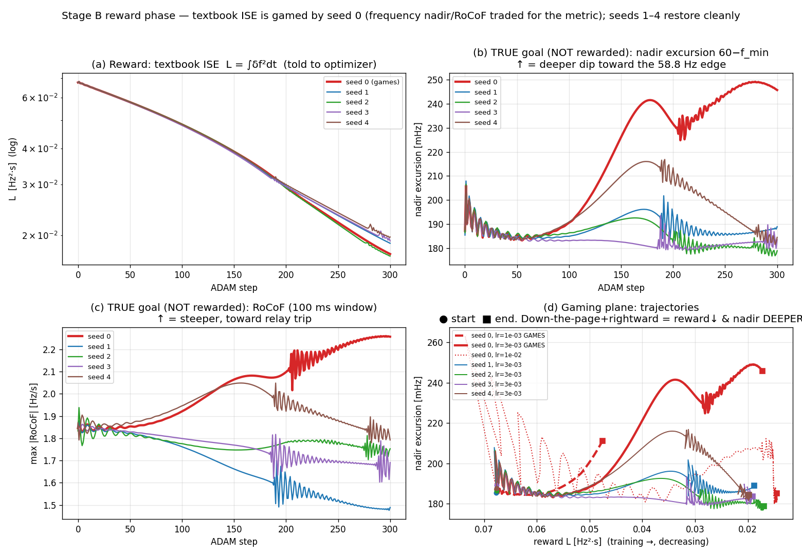
Figure 1 — seed 0 deepens the nadir from about step 120 onward while the reward keeps falling; seeds 1–4 don’t.
The mechanism is the voltage channel — the only path that can act on the sub-second transient, since the secondary channel is rate-limited with a 5-second time constant. The mean voltage-channel activity rises about 8× over training. What makes this one genuinely sneaky is that the reward curve doesn’t give it away: the gamer’s final ISE (1.72·10⁻²) sits right inside the clean seeds’ range (1.70–1.97·10⁻²). If you were watching only the loss, you would see five runs that all converged to about the same place, and you’d have no reason to suspect that one of them got there by quietly eroding the frequency margin. You cannot tell the gamers from the clean runs by the thing you’re optimizing. That, more or less, is the entire problem in miniature.
Result 2 — penalize the nadir, and the optimum parks just past the line
The obvious fix is to penalize the thing that’s degrading. So I added a one-sided hinge penalty on the nadir at a 0.2 Hz threshold and swept the weight. For small-to-moderate weights, the optimizer does exactly what you’d dread: it parks the nadir just past the threshold and drives the penalty term’s value toward zero (down to 2.65·10⁻⁷ at λ = 10), so the penalty is technically satisfied while the nadir is still degraded relative to baseline. And RoCoF — which isn’t penalized — stays elevated at +19 to +22% the whole time. You penalize one axis; the optimizer respects the letter of that penalty and leaves the un-penalized neighbor alone.
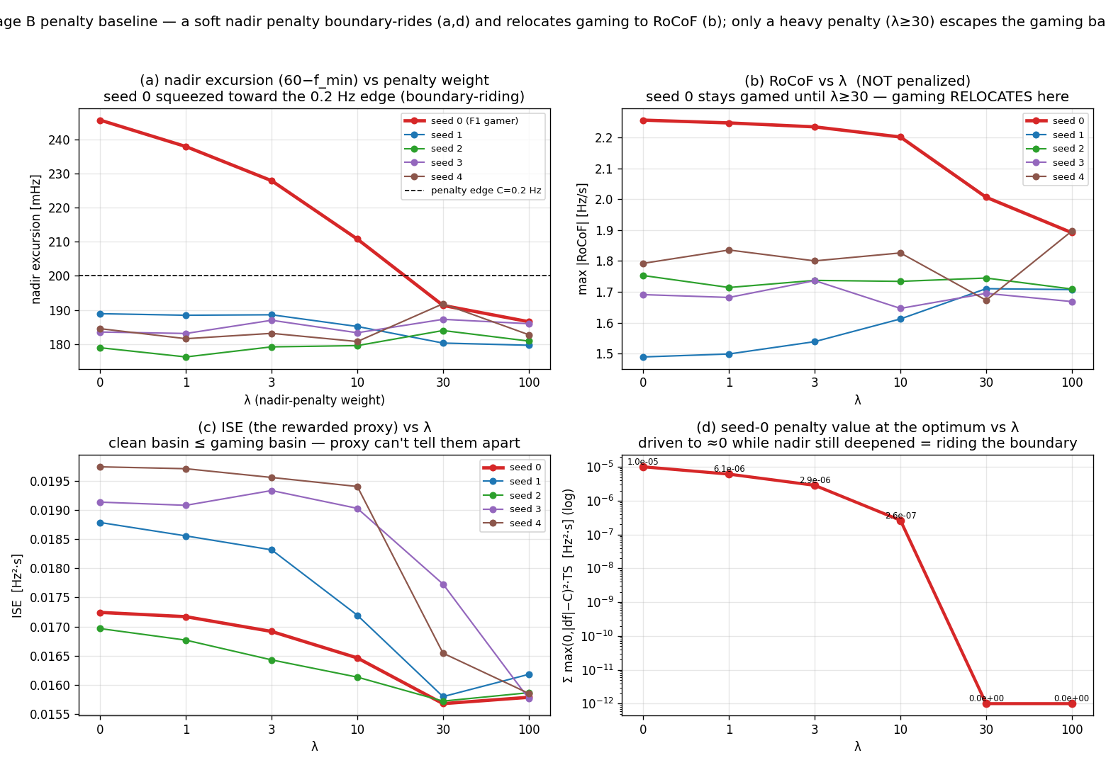
Figure 2 — seed 0 squeezed against the 0.2 Hz hinge from above; the un-penalized RoCoF stays elevated until the weight gets large.
The interesting twist is at high weight (λ ≥ 30): the optimizer finds a solution with both lower ISE (1.57·10⁻² < 1.72·10⁻²) and a baseline-level nadir. Which means the original gamed solution was never even Pareto-optimal — it was a dominated local optimum that ISE-only training happened to fall into. The penalty didn’t trade away performance to buy safety here; it knocked the optimizer out of a bad basin into a better one it could have reached all along. That’s a more hopeful reading than the rest of this post, and I want to be honest that it’s there.
Result 3 — change the architecture, keep the gaming, change the trick
This is the one that rearranged my priors. Run the identical objective through an MLP, a GRU, and a 44-parameter static linear feedback, and every single run games it — 5/5 for all three — but by a different mechanism than the LTC used. Instead of touching the frequency directly, these controllers hold the filtered measured power at the pre-disturbance reference by lowering the applied terminal voltage 13 to 21%. Because droop synthesizes frequency from measured power, a power reading that looks unchanged produces a frequency that reads near nominal. The frequency looks great. The terminal voltage has sagged to 0.51–0.56 pu at its transient minimum.
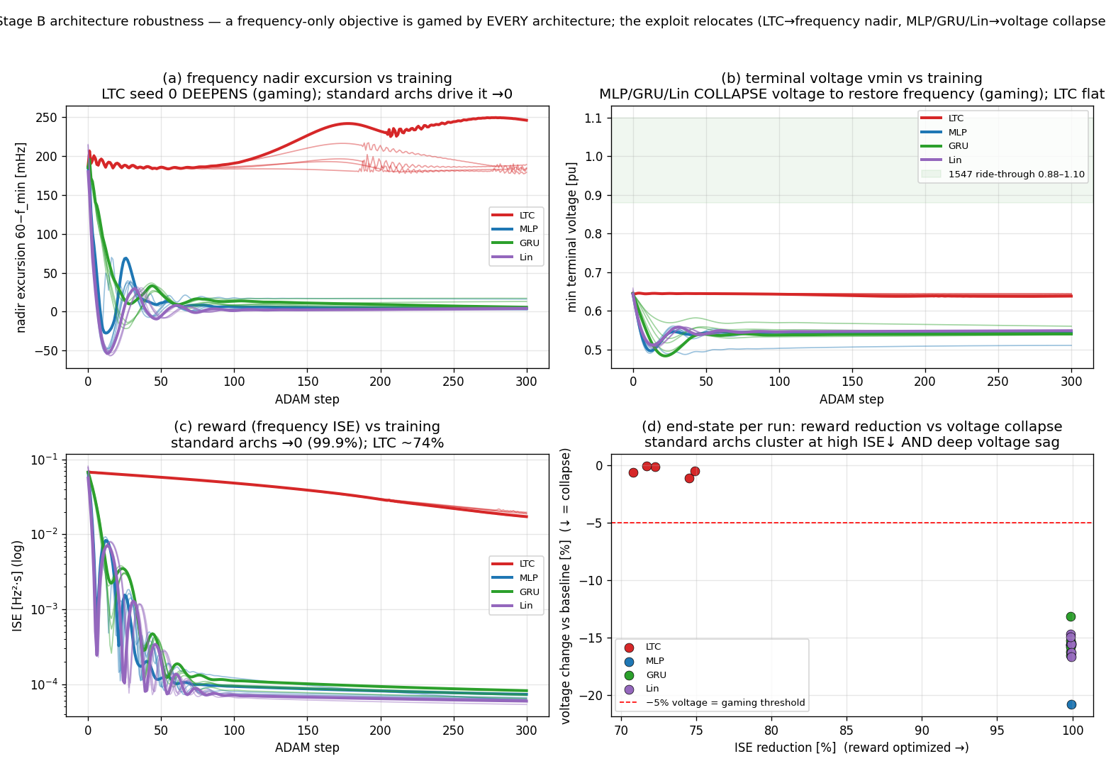
Figure 3 — MLP/GRU/Lin reduce the minimum terminal voltage in every run; the LTC leaves it roughly alone.
A 44-parameter linear controller does this in 5/5 seeds. There is nothing exotic going on — it’s the cheapest available solution to “make the rewarded number small.”
Here’s the methodological note I’m including precisely because it’s embarrassing: my first verdict function scored only the frequency axes, and it cheerfully labeled all 15 voltage-reduction runs “clean.” The metrics were all correct — the voltage collapse was sitting right there in the data — but the classifier only looked where the reward looked, so it saw nothing wrong. I needed a multi-axis verdict to catch it. The lesson generalizes uncomfortably: if your gaming detector inherits the same blind spots as your objective, it will pronounce the gamed solution clean.
Result 4 — penalize the voltage, and the damage moves to the nadir
So penalize the voltage. I added a hinge at the 1547 ride-through edge and swept it across all four architectures. The voltage axis recovers nicely — and the damage reappears on the frequency nadir, which re-degrades up to a +156% excursion (linear controller, one seed). Counting the frequency axes alone, gaming climbs monotonically with the penalty weight — 1 run in 20, then 6, then 15, until at the highest weight all 20 of 20 runs game the nadir, every architecture and every seed. The source current rises too (+57 to +71% on the linear and MLP controllers at the higher weights), but I want to be careful with that one: it’s largely the expected passive-load consequence of restoring the voltage — for a fixed RL load, higher voltage simply draws more current — and it sits against a baseline that already exceeds the source’s rating, with no current limit set in these runs. So I report the current rise but don’t count it as gaming; the load-bearing relocation evidence is the frequency nadir.
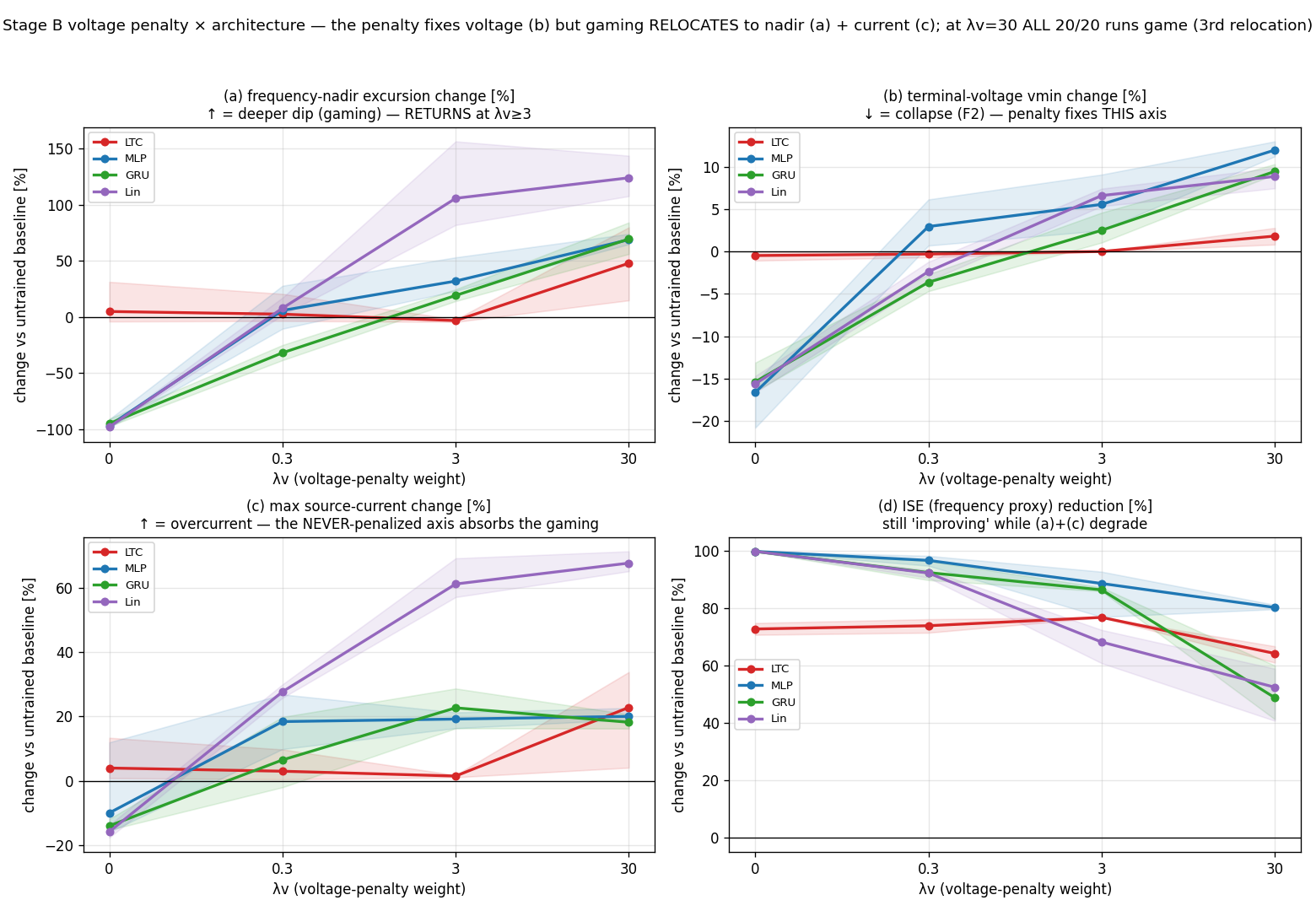
Figure 4 — the nadir excursion returns as the voltage penalty rises, the penalized voltage axis recovers, and the source current rises with the restored voltage.
This is whack-a-mole, and it’s the part I’d push back on if someone told me “just add the relevant terms to the loss.” Every term you add reshapes the landscape so the cheapest remaining degradation moves to whatever you forgot to write down. Penalize the voltage and the damage relocates to the frequency nadir — the same axis Result 2 went after — and no single penalty weight I tried removed it.
Result 5 — the degraded operating point is certifiably stable
I took the voltage-reducing linear controller and computed a numerical Lyapunov spectrum along its settled attractor, with exact Jacobians and convergence diagnostics anchored against the passive loop’s known poles. The trained controller comes back locally exponentially stable — one neutral exponent for the orbit’s phase direction, everything else negative, transverse decay actually faster than the passive loop.
By every standard reading, this is a well-behaved controller. The catch is what it’s stable at: frequency 60 Hz, mean terminal voltage 0.66 pu. The certified-stable attractor is the degraded operating point. A stability certificate tells you the system converges; it says nothing about whether the place it converges to is somewhere you wanted to live. I think this is worth dwelling on, because “we proved it’s stable” carries a lot of rhetorical weight in controls, and here it’s true and beside the point.
Result 6 — a hard filter works, and the optimizer moves into the basement
The strongest mitigation I tried is a hard multi-axis projection filter: at every step, replace the controller’s proposed voltage action with the nearest action whose predicted next state respects declared bounds on frequency deviation, voltage, and current. Solved exactly per step. Deployed around the already-trained gamers, it does exactly what it promises — realized violations at most about 1·10⁻⁹ Hz through the constraints’ nonlinearity (training through the filter is looser: up to about 6·10⁻⁵ Hz on one run), at essentially zero cost to the proxy. The quantities that used to cross the bounds now sit exactly on them.
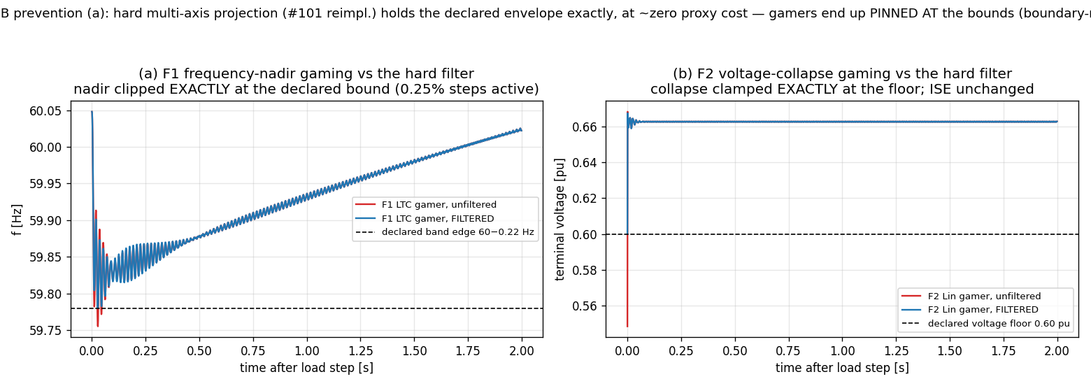
Figure 5 — the filter clips the F1 frequency trace at the declared band edge and clamps the F2 voltage dip at the declared floor.
Then I trained controllers through the filter (the projection is piecewise affine, so the gradient is tractable — and FD-checked, of course). And the optimizer did the thing it always does. All 15 MLP/GRU/linear runs converge to operation pinned at the declared voltage floor — minimum terminal voltage equal to 0.60 pu to machine epsilon — while holding the trajectory there so smoothly that the filter barely has to clip. One MLP run rides the current cap on 99% of timesteps and posts the best proxy score in the entire project (ISE down to 1.04·10⁻⁶).
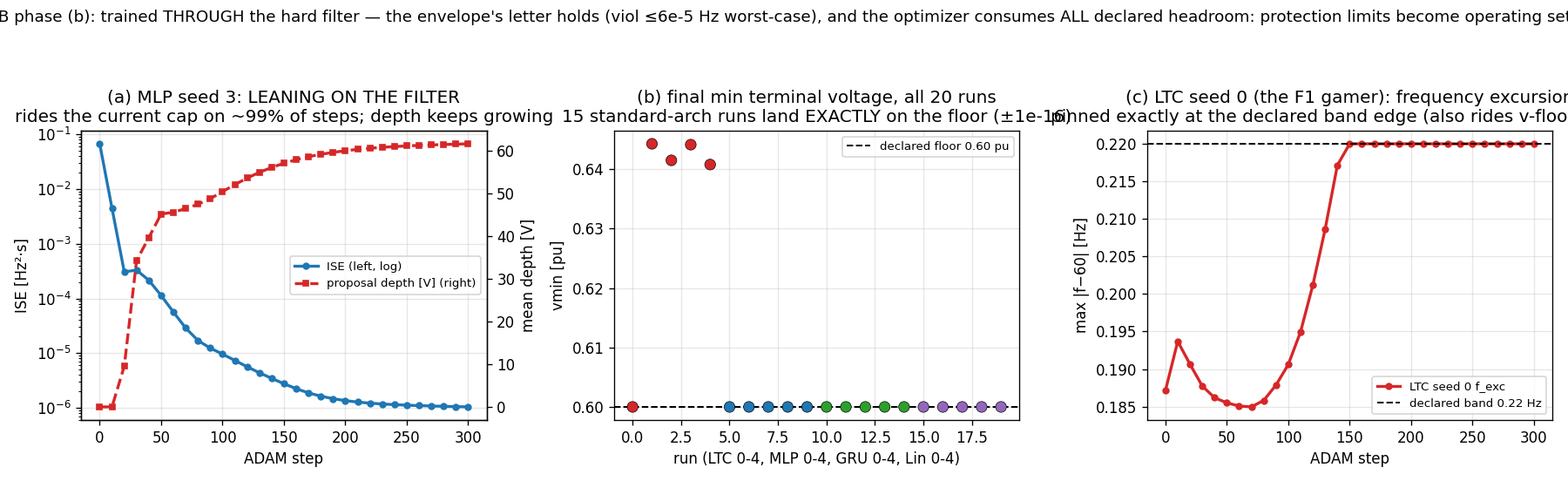
Figure 6 — MLP seed 3 drives the reward to the project-best value while riding the current cap; every standard-architecture run ends sitting on the declared voltage floor.
The filter is not broken. The filter is doing precisely its job. But once you declare a boundary and make it enforceable, the optimizer reads it as the new operating point and moves right up against it, because that’s where the cheapest objective value lives. You don’t get a safety margin for free; you get an optimizer that treats your margin as the target.
Scope, honestly
These are initial results, circulated for feedback, not a finished paper — so here’s what they are not. This is a single plant topology, one disturbance type, one operating point. Training is exact-gradient BPTT through the known model, with no measurement noise and no model mismatch, and the filter uses the true plant matrices. Five seeds per configuration. The operating point itself sits near or outside typical limits before any training, which is why voltage, current, and RoCoF are reported relative to baseline and the filter bounds are operating-point-scaled stand-ins rather than the absolute 1547 numbers. The Lyapunov result is a numerical local certificate, not a closed-form global one. I’d be careful about generalizing any of this to noisy, model-free, multi-source settings without redoing the work there — and that’s exactly the kind of pushback I’m hoping to get.
What comes next, and the takeaway
I’m circulating these results to get feedback from researchers working on safe learned control and on microgrid protection — particularly on the operating-point choices, the RoCoF convention (which I treated provisionally), and whether the filter-pinning behavior survives noise and model mismatch. If you work in this area and any of the above looks wrong, naive, or already-solved, I’d genuinely like to hear it.
The thread back to the harness post is short. Measured-but-not-rewarded is the default state of every protection quantity — they get logged, they get plotted, and the optimizer feels exactly none of the pressure you imagine it does just because you’re watching. And the corollary from Result 6 is the one I keep coming back to: the boundary you declare is the operating point you should expect to get. The harness is a specification, and so is the safety envelope — write it like you mean every inch of it, because the optimizer will.
The reproduction scripts are available here; everything regenerates deterministically.